Ray Tracing: Revisited Part 3

In this part of the project, we had to implement;

• Transformations
• Instancing
• Multisampling
• Depth Of Field
• Area Lights
• Motion Blur
• Glossy Reflections

I’m delivering this part in OdtuClass today (10/05/2021) because I could not debug some problems that I was facing. I didn’t want to publish an unfinished work so I tried to debug them all night. They were very silly mistakes which I’m going to explain shortly.

Transformations

Firstly we had to implement transformations. We have three different transformation types;

• Translation
• Rotation
• Scaling

Just like we saw in class and in Ceng477, these transformations are described with 4×4 matrices. And in order to implement a sequence of transformations, we just multiply them from right to left.

I had to do a minor refactoring to implement transformations on scene objects. Until now, I was dealing with triangles, spheres and meshes without any OOP concepts. So firstly, I created a Base Object class and stored three matrices and a virtual function like this(of course I’m simplifying the code a little bit);

class Object
{
public:
    glm::mat4 transformationMatrix;
    glm::mat4 transformationMatrixInversed;
    glm::mat4 transformationMatrixInverseTransposed;

    virtual bool Intersect() = 0;

};

So, why I’m storing transformationMatrixInversed and transformationMatrixInverseTransposed?

When testing for intersections, I do not transform object vertices or objects into world coordinates. Instead, I’m transforming the ray to local coordinates of the object. In order to do this, I transform the ray using inversed version of transformation matrix.

Secondly, I also need to transform normals for light calculations or reflections. I had two choices here;

• Transform lights to local coordinates
• Transform normals to world coordinates

I liked the second option more and transformed the normal vectors of intersections to world coordinates. For that, I’ve used inverse transpose of transformation matrix

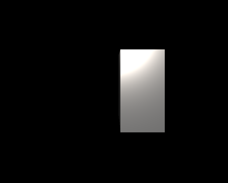
After arrangements, I had my first results;

simple_transform.png

ellipsoids.png

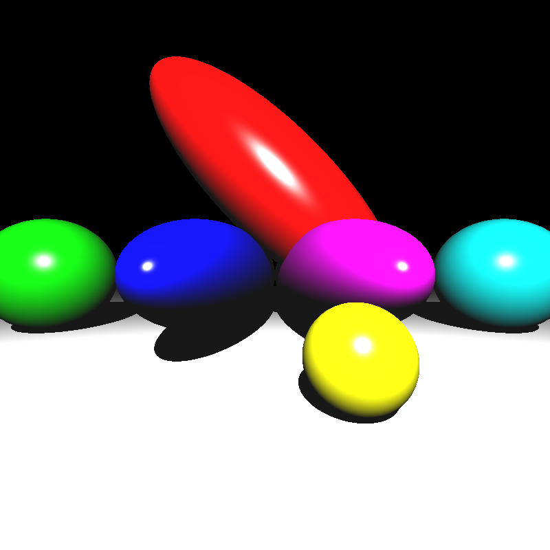
According to this result, I assumed that I had correctly implemented transformations and moved on to the next step, Instancing.

Instancing

Just like we’ve learned in class, we need instancing to save some memory. We can use same objects and just by instancing create multiple versions of them and put them into different positions and change their orientations with different transformations without allocating more memory. That’s the point of instancing as far as I’ve understood.

I’ve created a new child class of Object which is MeshInstance. Mesh instance behaves just hold a pointer to the Mesh object and uses its data for intersection computations. I don’t want to give my results about instancing here because they are being used with different techniques which I’m going to explain after this part. So my implementation can be seen in those parts

Multisampling

Multisampling is for increasing the accuracy and quality of the results. And it also makes it easier for us to implement some visual effects. What I did was dividing each pixel that I’m going to process into N uniform parts and create rays for each of them. So I’ve implemented jittered sampling. But here, I had to create random numbers. I also saw that I’ll need a lot more random variables later, I created a random number generator class;

class RandomGenerator
{
private:
    float rangeFrom;
    float rangeTo;
    std::random_device randomDevice;
    std::mt19937       generator;
    std::uniform_real_distribution<float> distr;

public:
    RandomGenerator(float from, float to)
    {
        rangeFrom = from;
        rangeTo   = to;

        generator = std::mt19937(randomDevice());
        distr     = std::uniform_real_distribution<float>(rangeFrom, rangeTo);
    }

    float Generate()
    {
        return distr(generator);
    }
    
};

So I’ve used this class for creating random positions on each part inside the pixel.

For filtering, I’ve used gaussian filtering. I assigned weight on each created ray according to its distance to the center of pixel. I’ve created this utility function to deal with it;

inline float GaussianWeight(float x, float y, float stdDev)
{
    return (1/(2*M_PI*stdDev*stdDev)) * std::pow(EULER, (-1/2)*((x*x + y*y)/(stdDev*stdDev)));
}

I also don’t want to share results in this part because I need to explain visual effects first.

Depth of Field

Finally, after implementing multisampling, I first dived into depth of field part. What I needed to do was just adding focusDistance and apertureSize variables to the camera and create random variables for location in the lens.

I made use of this while creating primary rays. By using the equations in our slide, I calculated new rays coming from the lens. This is the result I had;

spheres_dof.png (rendered in 6.33371 seconds – 100 samples)

Yes, it is a bit noisier than the correct image. I did not find what I need to do to make it better. But if I increase sample size to 900;

spheres_dof (rendered in 64.469 seconds – 900 samples)

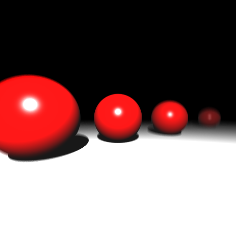
It becomes a little bit better at the cost of being rendered a lot slower.

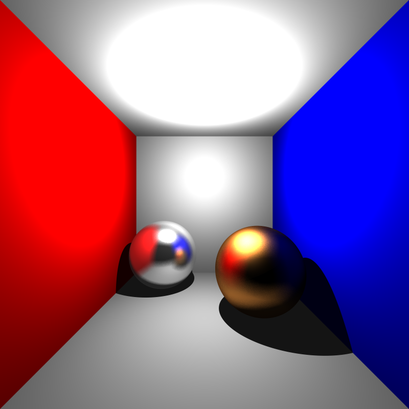
Area Lights

I created a new light structure for area lights. Area lights are used to create soft shadows. In area lights, we make an orthonormal basis(I make it in constructor of area light since we don’t transform it) using the normal vector. We also calculate random positions in the surface of area light and use it as the light.

Secondly, we don’t use intensity just like we do in point light. We do a different calculation for irradiance. We need to take;

• vector from intersection point in object surface to random position in area light surface and area light surface normal and cosine of the angle between them
• radiance value of area light
• area value of the light
• distance between random position in light and intersection point

While computing the cosine value of that angle that I’ve mentioned above, we need to take its absolute value because if we don’t, light will not illuminate other side of the area light.

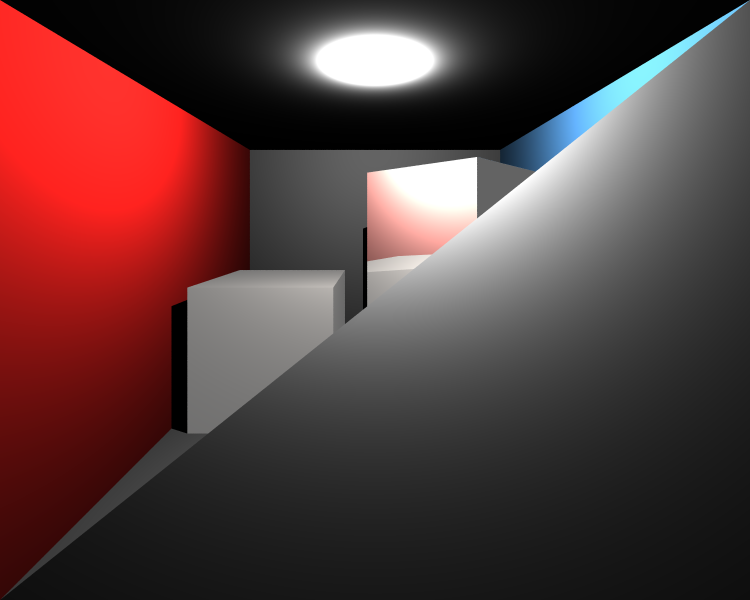
Here, I had a really annoying problem. That’s it;

cornellbox_area.png wrong

You see that spheres look ok but there is a problem in ceiling. I was actually thinking about delivering this part of the project yesterday but solving this problem took nearly 3-4 hours.

The problem was not about my area light implementation or calculations, problem came from my filtering code. The problem was I was clamping pixel values between 0.0 and 1.0(I don’t use 8 bit unsigned integers, I use floating numbers between 0 and 1) when computing pixel of traced ray. But this was creating a problem while taking weighted average coming from different samples. So, I stopped clamping it in raytracing function and clamped the pixel after filtering operation. This corrected the problem;

cornellbox_area.png (rendered in 11.9647s – 100 samples)

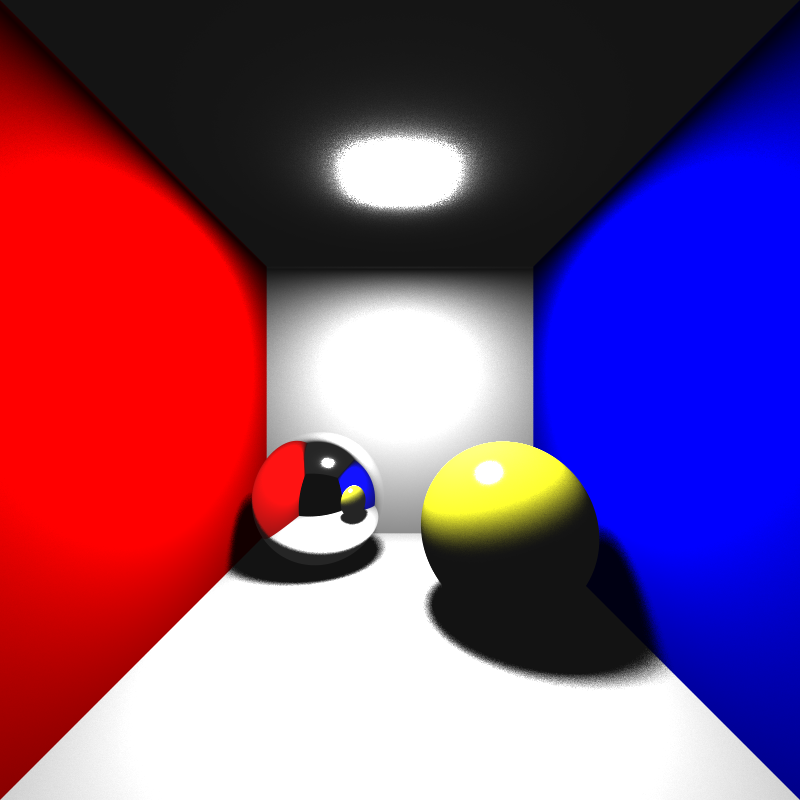
Again it is a bit noisier than the example, but it becomes a lot better if we increase sample number to 900 😀

cornellbox_area.png (rendered in 103.478s – 900 samples)

Motion Blur

In this part, we are making use of transformations and random variables between 0.0 and 1.0. For simplicity we only had to implement translations. I gave a random time variable between 0.0 and 1.0 to each sample ray and when calculating intersections, I translated moving objects according to the time.

Here are the results;

cornellbox_boxes_dynamic.png (rendered in 75.7427 seconds – 900 samples)

dragon_dynamic.png (rendered in 148.609s – 100 samples)

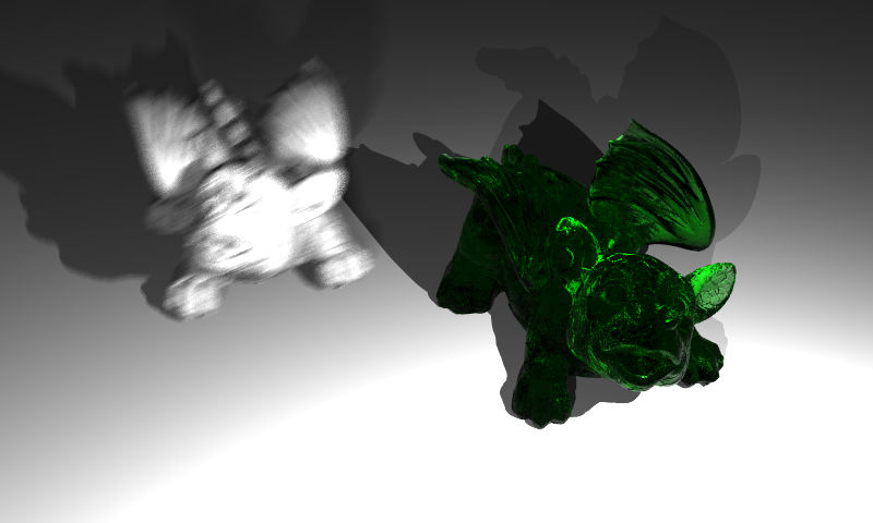
These pictures also show that my instancing implementation is correct. By the way green dragon looks like a jelly, I really liked it :D.

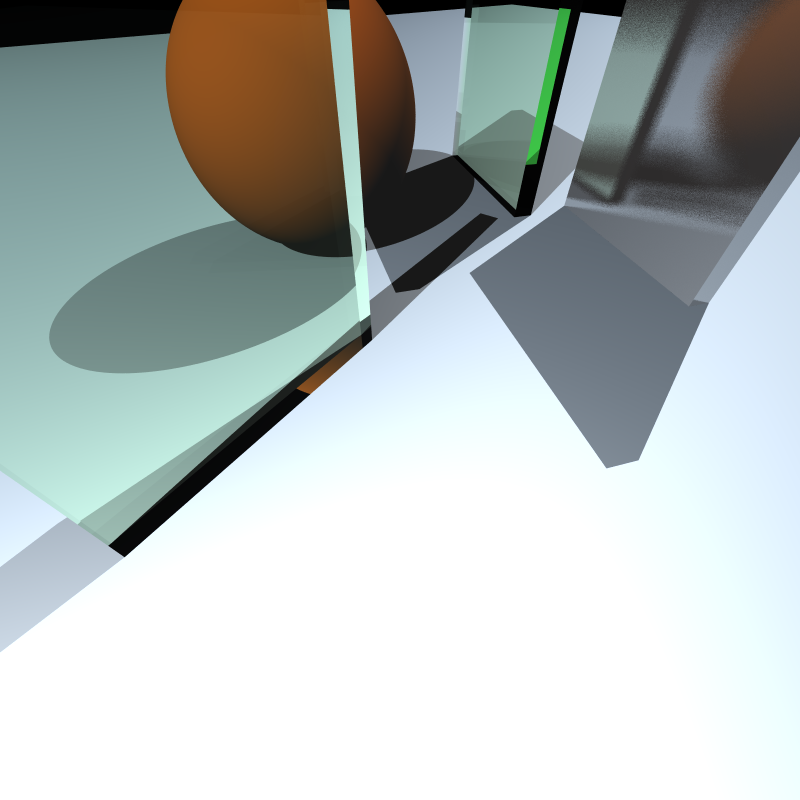
Glossy Reflections

Lastly, I had to implement glossy reflections. It is for simulating imperfect reflections. Again I used random variables, created an orthonormal basis with reflected ray direction and changed the direction of the reflected ray using the vectors I obtained while creating the orthonormal basis.

I made use of roughness parameter here for determining how strong imperfect reflections are. This parameter only applies for mirror and conductor type of materials. Here are my results;

cornellbox_brushed_metal.png (rendered in 35.3315 seconds – 400 samples)

These balls look like the ones they put onto pine trees.

metal_glass_plates.png (rendered in 10.6414 seconds – 36 samples)

Debugging Process

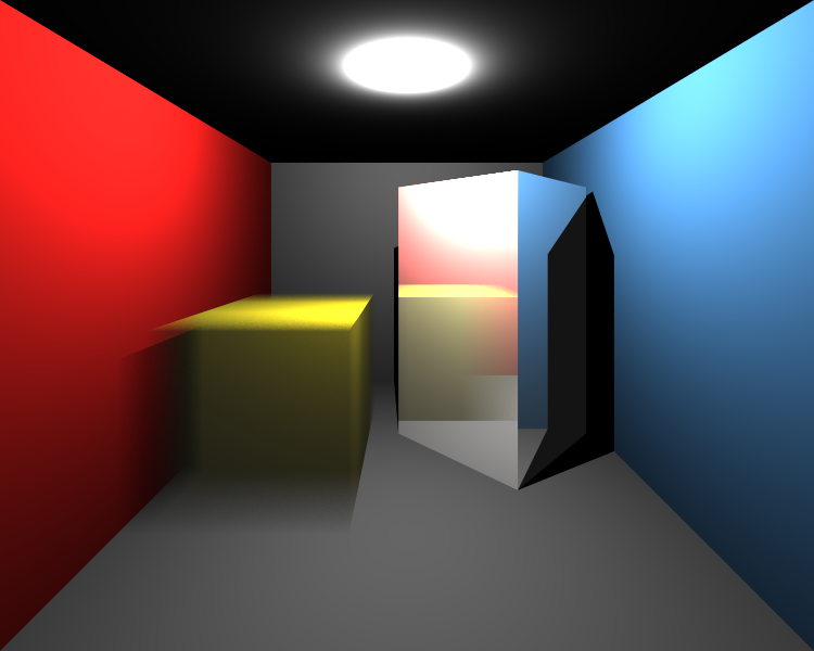
I could not obtain these images above easily. I struggled and panicked a lot :D. I recorded some of my bad results. For example, in cornellbox_boxes_dynamic image, I was getting this;

cornellbox_boxes_dynamic.png

I sat down and started thinking why I get this image. During this process, I have learned a way to debug image errors. It may or may not be a good way but It helped me a lot. I may learn better ways in the future since I’m a beginner right now :D.

So, what I do when I get wrong images?

• I start removing suspicious objects from the scene. Maybe I can understand what causes the problem
• Play around with xml a litle bit more
• If I cannot understand where is the problem, I switch debugging mode and control with gdb and firstly try to answer these questions:
  • Do I parse xml file correctly?
  • Are my calculations correct?
• If everything seems correct, then I first make calculations on paper and trace specific rays with gdb.

I really hate the last option. It is hard for me so I don’t bother dealing with gdb first. Trying other options before this one is better.

For example for the above image, instead of starting hard debugging process, I just started removing some objects and got this;

wrong cube

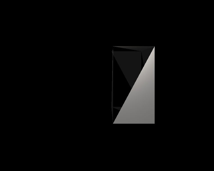
I have a cube but it looks weird. So there is another problem here. By looking at the cube, I saw that it only renders half of the faces of the cube.

So there is a problem in parsing ply files. But where? Since ply file of cube is not huge, I looked at it in text editor and saw that in the file, faces have 4 points instead of 3. But in my ply parsing code, I just assumed that faces can only be triangles. So added parsing code for faces having 4 points and;

correct cube

I got this image above. By the way I also deleted some transformations applied on the cube thats why it is not rotated. So I solved a problem on the way. But why I’m getting the first picture (a gray illuminated plane).

This time, I restored the xml file and started playing with faces of meshes and I got this image;

another image

So it seems that one plane is blocking our sight. This must mean that we should not render this plane at all while looking from here. I had some “educated” guesses about the solution but in order to be sure, I examined vertex position of the faces of that particular plane.

Yeah, vertices are in clockwise order. So surface normal of the plane points away from us. This means that this image want us to implement backface culling.

So, I implemented backface culling and disabled it for dielectrics(for obvious reasons) and it worked.

From the image we can see that cube on the left is not yellow, so there is a problem while assigning material to mesh instance (good guess, corrected)

And also if you look at the reflections on the rightmost cube, you can see that it is not correct too. So this means there might be a problem while translating surface normals since we need them to create reflected rays (good guess, corrected)

I do not want to use extra effort for nothing. If I dived into gdb quickly, I could not understand all these problems that fast. That’s my approach for handling errors. Maybe it is not the best way but it helped me a lot. I got a lot more errors then the ones I’ve mentioned but this blog is going to be really long if I try to explain all of them. But they are all similar.

Conclusion

Another part is finished. I’m happy with the results. Quality of my images are a lot better and of course they are rendered a lot slower. I’ve learned a lot of things. Especially I think my problem solving skills are increasing as well.