Raytracing Revisited: Part 6

In this part, we have added Bidirectional reflectance distribution function (BRDF) to our ray tracers. This homework was simpler than the previous work we had done. We have added;

• Phong
• Modified Phong
• Blinn – Phong
• Modified Blinn – Phong
• Torrance – Sparrow

Models as BRDF functions. I started with adding new functions for reading BRDF information from our xml files. After I finished properly reading the information, I started my implementation.

There are two principles we need to obey;

1. Helmholtz reciprocity principle => f(x,wi,wo) = f(x,wo,wi) (our ray tracers are based on this principle I guess :D).
2. Energy conservation principle => we cannot generate extra energy.

As we learnt in class, our reflected radiance is calculated like this;

how we compute reflected radiance

Actually, before this homework, we were using blinn – phong shading model so my code was designed according to that. So I changed my code a little bit here.

I added a new function f(x, wi, wo) to my base light class to give modified values of diffuse and specular reflectances according to the BRDF model that we were using. And I used this function to calculate the color using the above equation.

Original Phong

Here, we are using the angle between the perfect reflection of wi across the surface normal and wo direction. We cannot normalize this because it is already energy conserving. Here are my results for original phong inputs;

brdf_phong_original.png 54.592ms

Modified Phong

We do not divide specular reflectance with the cosine of angle between wi and surface normal and get modified phong model. We can normalize it. Here are my results;

phong_modified.png 51.787ms

Here is the normalized result;

phong_modified_normalized.png 62.339ms

Original Blinn – Phong

This is the shading model that we have been using. We calculate a half vector of wi and wo and look at the angle between this vector and the surface normal. That’s the idea of blinn-phong shading model. Here is my result;

brdf_blinnphong_original.png 69.346ms

Modified Blinn – Phong

Just like in the modified phong case, we do not divide the specular reflectance with the cosine of angle between wi and surface normal. We can normalize this model too. Here are my results;

brdf_blinnphong_modified.png 57.791ms

Here is the normalized output;

brdf_blinnphong_modified_normalized.png 51.875ms

Torrance – Sparrow

In this model, we use fresnel reflection and treat the surface like it is made up from micro-facets. So in this model, we are using;

• Distribution for probability of angle alpha ( angle between half vector and normal, we have used Blinn’s distribution here)
• Geometry term (shadowing and masking properties of micro-facets are modelled with this term)
• Fresnel term (Schlick’s approximation is said to be used)

With this configuration, here is my result;

brdf_torrancesparrow.png

We can see that there is a little problem here because it does not match with the provided output. Thanks to the post I saw on ODTUClass written by our classmate, I understood that instead of using schlick’s approximation, we need to use the fresnel calculation that we have implemented for conductors. After changing the code according to that, here is my output;

brdf_torrancesparrow.png 54.091ms

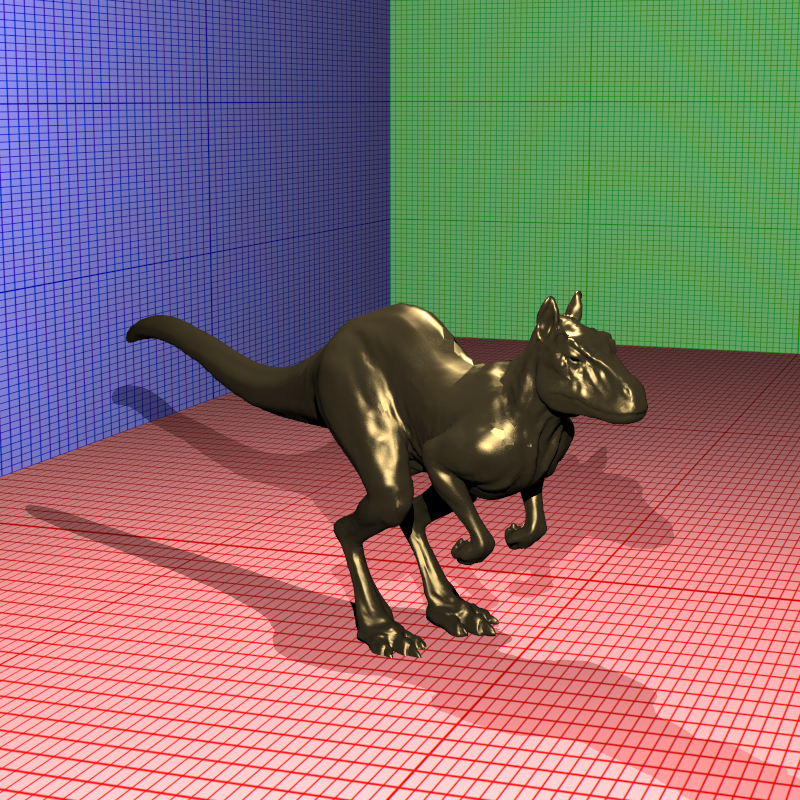
Killeroo Scenes

Here I had some problems :D. I thought this would be one shot one kill type of homework but I was wrong. The first problem was I did not implement my raytracer to produce more than one image in one run. I had to implement it before but I forgot. First of all, I ensured rendering multiple cameras at once.

Secondly, when I ran my raytracer I got this;

weird killeroo

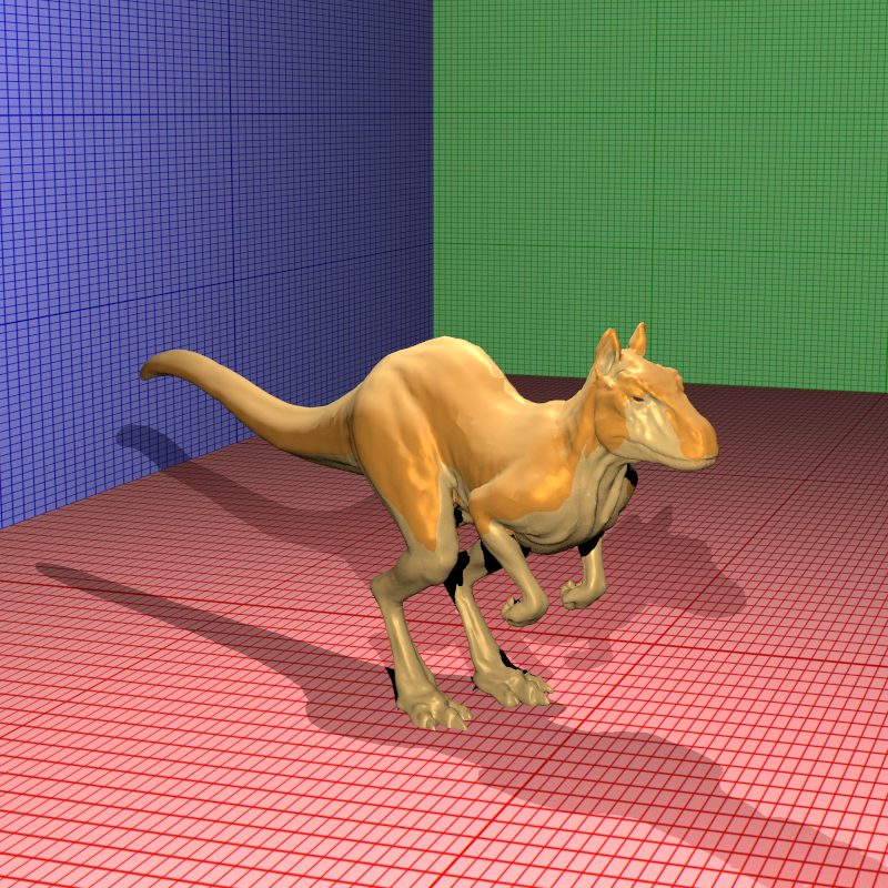
I had no idea what was happening here at first (this pattern was cool though :D). Then, I carried on my usual debugging procedure. I started playing around with xml first and I changed degamma on killeroo mesh to false and saw the result;

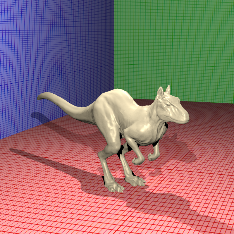
The pattern has gone. So I have a problem when I’m modifying diffuse and specular reflectances.

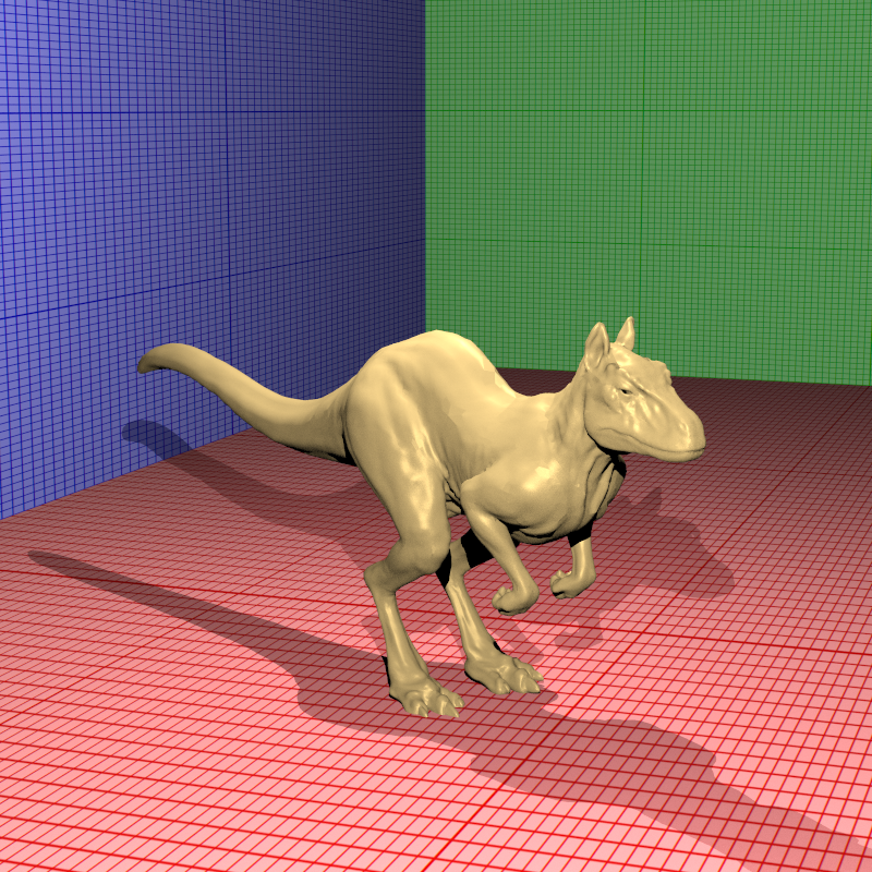
In my code, I was traversing all light sources and giving them the intersection reports, material properties etc.. But I was giving reflectance coefficients as references. So that I was using degamma multiple times if I had more than one light sources. That was the case.

So I corrected this mistake and got my results;

killeroo_blinnphong.png 5.31396s

killeroo_blinnphong_closeup.png 11.9519s

killeroo_torrancesparrow.png 3.6343s

killeroo_torrancesparrow_closeup.png 12.506s

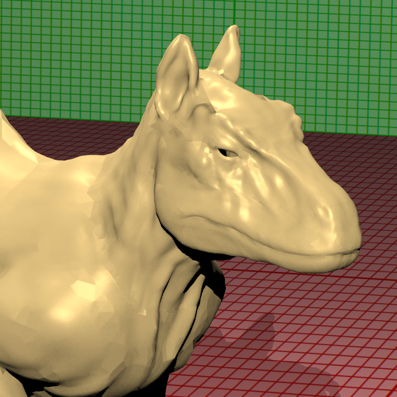
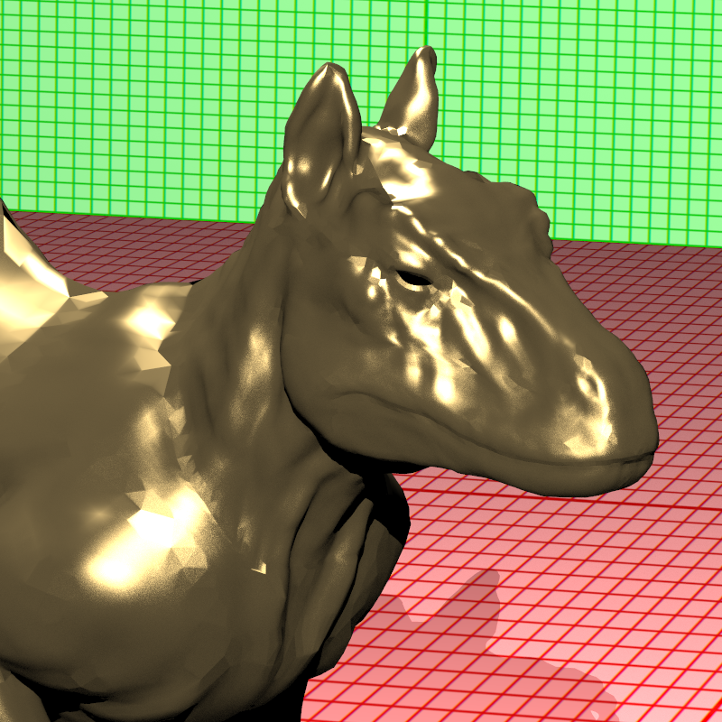
Conclusion

I have a little problem to be solved but it is not about brdfs, I guess it is because of how I implement soft shading. I realised the problem by looking closer to killeroo scenes, few amount of triangles do not seem smooth. I will solve this problem. I looked at the situation where I implemented texturing and saw that there was no problem about soft shading with killeroo scene. I must have broken something while calculating normals but could not find for now.

Besides that, in this homework we have implemented BRDF models to our raytracers and I also have done some debugging and code cleaning.